Coursera ML(5)-Logistic Regression and Regularization with Python

线性回归算法,可用于房屋价格的估计及股票市场分析。 Logistic Regression (逻辑回归)是当前业界比较常用的机器学习方法,用于估计某种事物的可能性。比如某用户购买某商品的可能性,某病人患有某种疾病的可能性,以及某广告被用户点击的可能性等。相关公式推导在这里


Stanford coursera Andrew Ng 机器学习课程编程作业(Exercise 2),作业下载链接貌似被墙了,下载链接放这。http://home.ustc.edu.cn/~mmmwhy/machine-learning-ex2.zip

预备知识

这里应该分为 正常、过拟合和欠拟合,三种情况。

  • Cost Function
  • Gradient Descent

  • Grad

后边有一个$\frac{\lambda}{2m}\sum_{j=1}^n \theta_j^2$和$\frac{\lambda}{m}\theta_j$小尾巴,作用就是进行 Regularization,防止拟合过度。

Logistic Regression

题目介绍

  • you will build a logistic regression model to predict whether a student gets admitted into a university.(根据各科目分数预测该学生是否能录取)
  • For each training example, you have the applicant’s scores on two exams and the admissions decision.
  • Your task is to build a classi cation model that estimates an applicant’s probability of admission based the scores from those two exams.
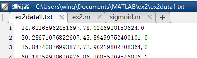
dataset

python code

1
2
3
4
5
6
7
8
9
10
11
12
13
14
15
16
17
18
19
20
21
22
23
24
25
26
27
28
29
30
31
32
33
34
35
36
37
38
39
40
41
42
43
44
45
46
47
48
49
50
51
52
53
54
55
56
57
58
59
60
61
62
63
64
65
66
67
68
from numpy import *
import matplotlib.pyplot as plt
from scipy import optimize

def init(path):
X,y = load_dataset(path) # 调用底下那个东西
m, n = shape(X)
initial_theta = zeros(n + 1)
return X,y,m,n,initial_theta

def load_dataset(path):
data = loadtxt(path, delimiter=',')
X = data[:,:2]
y = data[:, 2]
return X,y

def plotData(X,y):
plt.plot(X[y==1][:,0],X[y==1][:,1],'k+',linewidth=2,)
plt.plot(X[y==0][:,0],X[y==0][:,1],'ko',color='y',linewidth=2)
plt.xlabel('科目一成绩', fontproperties='SimHei')
plt.ylabel('科目二成绩', fontproperties='SimHei')
plt.title('分数与录取的关系', fontproperties='SimHei')


def sigmoid(X, theta):
return 1 / (1 + exp(-dot(X, theta)))

def get_cost(theta, X, y):
J = sum((-y*log(sigmoid(X,theta)) - (1-y)*log(1-sigmoid(X,theta))))/len(X)
return J

def get_grad(theta, X, y):
return (sigmoid(X,theta) - mat(y))*X*(1/m)

def plotDecisionBoundary(theta, X, y):
plotData(X[:, 1:3], y)
if X.shape[1] <= 3:
plot_x = r_[X[:,2].min()-2, X[:,2].max()+2]
plot_y = - (theta[1]*plot_x + theta[0])/theta[2]
plt.plot(plot_x, plot_y)
plt.axis([30,100,30,100])
plt.legend(['Accepted', 'Not Accepted', 'Decision Boundary'])
plt.show()
else:
pass


def predict(theta, X):
prob = sigmoid([1,45,85] , result[0])
return prob

if __name__=="__main__":
path = 'C:\\Users\\wing\\Desktop\\machine-learning-ex2\\ex2\\ex2data1.txt'
X,y,m,n,initial_theta = init(path)
X = column_stack((ones(m), X))
cost = get_cost(initial_theta, X, y)
grad = get_grad(initial_theta, X, y)

# obtain the optimal theta
result = optimize.fmin_tnc(func=get_cost, x0=initial_theta, fprime=get_grad, args=(X, y))
get_cost(result[0], X, y)
# result = (array([-25.16131863, 0.20623159, 0.20147149]), 36, 0)
# get_cost(result[0], X, y) = 0.20349770158947464
plotDecisionBoundary(result[0], X, y)
print('For a student with scores 45 and 85, we predict an admission ' \
'probability of %f\n'%predict(result[0], X))

# For a student with scores 45 and 85, we predict an admission probability of 0.776291

运行结果


最后进行了一个测试,如果一个学生两门考试成绩,一门45分,另外一门85分,那么他被录取的概率为77%。幸亏是在外国,在中国这分数,连大专都考不上。

Logistic Regression and Regularization

题目

  • Suppose you are the product manager of the factory and you have the test results for some microchips on two di erent tests.
  • 对于一批产品,有两个检测环节,通过检测结果判断产品是否合格。比如,宜家会有三十年床垫保证,那么如果确保床垫合格(用30年),我们只能通过一些检测,来推测产品是否合格。

python code

1
2
3
4
5
6
7
8
9
10
11
12
13
14
15
16
17
18
19
20
21
22
23
24
25
26
27
28
29
30
31
32
33
34
35
36
37
38
39
40
41
42
43
44
45
46
47
48
49
50
51
52
53
54
55
56
57
58
59
60
61
62
63
64
65
66
67
68
69
70
71
72
73
74
75
from numpy import *
import matplotlib.pyplot as plt
from scipy import optimize

def init(path):
X,y = load_dataset(path)
dataplot(X,y)
X = map_feature(X[:,0], X[:,1])
initial_theta = zeros(size(X[1]))
lam = 1
return X,y,initial_theta,lam

def load_dataset(path):
data = loadtxt(path, delimiter=',')
X = data[:,:2]
y = data[:, 2]
return X,y

def dataplot(X,y):
plt.plot(X[y==1][:,0],X[y==1][:,1],'k+',linewidth=2)
plt.plot(X[y==0][:,0],X[y==0][:,1],'ko',color='y',linewidth=2)
plt.legend([ 'y = 1','y = 0'])

def sigmoid(X, theta):
return 1 / (1 + exp(-dot(X, theta)))


def map_feature(x1, x2):
#X1, X2, X1 ** 2, X2 ** 2, X1*X2, X1*X2 ** 2, etc...

x1.shape = (x1.size, 1)
x2.shape = (x2.size, 1)
degree = 6
out = ones(shape=(x1[:, 0].size, 1))
m, n = out.shape
for i in range(1, degree + 1):
for j in range(i + 1):
r = (x1 ** (i - j)) * (x2 ** j)
out = append(out, r, axis=1)
return out

def get_cost(theta, X, y,lam):
hx = sigmoid(X,theta)
thetaR = theta[1:]
J = sum((-y*log(hx) - (1-y)*log(1-hx)))/len(X) \
+ (lam / (2.0 * len(X))) * (thetaR.T.dot(thetaR))
return J

def get_grad(theta, X, y,lam):
reg = (lam/len(y))*theta
reg[0] = 0
grad = X.T.dot(sigmoid(X,theta)-y)/len(y)+reg
return grad

def plotDecisionBoundary(theta,lam):
u = linspace(-1, 1.5, 50)
v = linspace(-1, 1.5, 50)
z = zeros(shape=(len(u), len(v)))
for i in range(len(u)):
for j in range(len(v)):
z[i, j] = (map_feature(array(u[i]), array(v[j])).dot(array(theta)))
z = z.T
plt.contour(u, v, z)
plt.title('lambda = %f' % lam)
plt.xlabel('Microchip Test 1')
plt.ylabel('Microchip Test 2')
plt.axis([-0.85,1.1,-0.85,1.1])
plt.legend(['y = 1', 'y = 0', 'Decision boundary'])
plt.show()

if __name__=="__main__":
path = 'C:\\Users\\wing\\Desktop\\machine-learning-ex2\\ex2\\ex2data2.txt'
X,y,initial_theta,lam = init(path)
result = optimize.fmin_tnc(func=get_cost, x0=initial_theta, fprime=get_grad, args=(X, y,lam))
plotDecisionBoundary(result[0],lam)

运算结果

  • 过拟合
    lambda=0。不考虑$\frac{\lambda}{2m}\sum_{j=1}^n \theta_j^2$和$\frac{\lambda}{m}\theta_j$,我们可以看到图像已经被拟合过度。这样的答案没有通用性
  • 欠拟合
    lambda=10,欠拟合会导致数据的很多细节被抛弃。
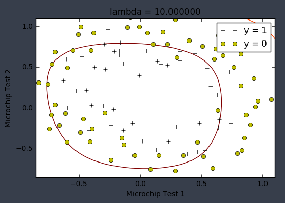
  • 拟合较好
    lambda=1,准确性到91%左右,这个准确率算低的了吧,还有很大上升空间。
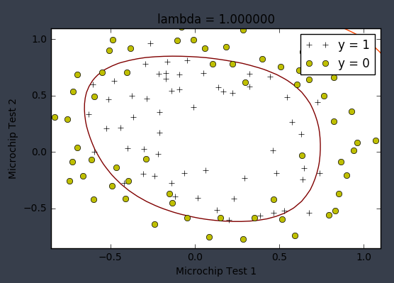
Summary

熊辉上课的时候,说机器学习需要调参数,参数很不好调,需要使用者对数据有极高的敏感度。

参数lambda就是这种感觉,感觉真的是乱调一通,然后就发现,诶哟,好像还不错。

参考链接:
scipy.optimize.minimize
Logistic regression
Machine Learning Exercises In Python, Part 3
machine-learning-with-python-logistic


以上

Coursera ML(5)-Logistic Regression and Regularization with Python

https://iii.run/archives/0d427e4d255f.html

作者

mmmwhy

发布于

2017-03-30

更新于

2022-10-30

许可协议

评论