相关概念 tf.nn.conv2d 函数tf.nn.conv2d(input, filter, strides, padding, use_cudnn_on_gpu=None, name=None)有六个参数,其中前面的四个比较主要。
input :输入图片,格式为[batch,长,宽,通道数],长和宽比较好理解,batch就是一批训练数据有多少张照片,通道数实际上是输入图片的三维矩阵的深度,如果是普通灰度照片,通道数就是1,如果是RGB彩色照片,通道数就是3,当然这个通道数完全可以自己设计。
filter :就是卷积核,其格式为[长,宽,输入通道数,输出通道数],其中长和宽指的是本次卷积计算的“抹布”的规格,输入通道数应当和input的通道数一致,输出通道数可以随意指定。
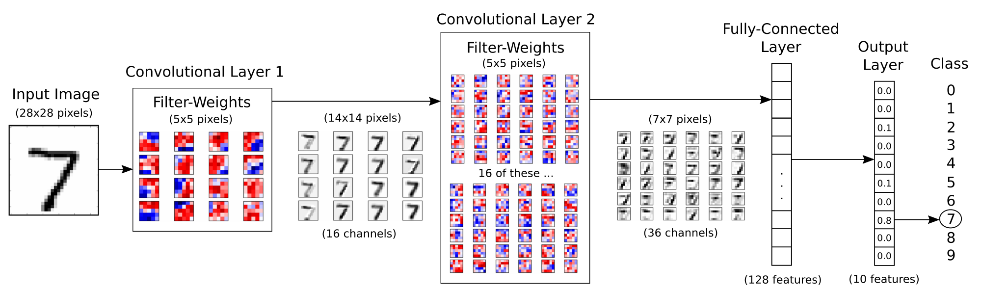
CNN
输入的图像在第一个卷积层使用 filter-weights 进行处理,获得16个新的图像,每一个对应一个卷积层中的 filter。 图片同时进行了 max pool ,由28 x 28 变成了 14 x 14 。
filter-weights ,这个词我也不知道该怎么翻译,作用是加强或者削弱图像的某些方面。 我们当然是希望这些filter能有一些sense,比如能感觉到 圈 或者 直线。
卷积层2
连接层
卷积算子初始化是随机的,因此此时的分类也是随机的,表现为正确率约为10%左右,预测和输入图像的真实值计算获得 交叉熵。 优化器自动将错误传回CNN当中去,并优化 算子参数(filter-weights),运算多次之后会发现分类正确率明显上升。
分层
输入层:用于数据的输入
卷积层:使用卷积核进行特征提取和特征映射
激励层:由于卷积也是一种线性运算,因此需要增加非线性映射
池化层:保留最显著的特征,提升模型的畸变容忍能力。
全连接层:图像中被抽象成了信息含量更高的特征在经过神经网络完成后续分类等任务。
输出层:用于输出结果
stride(步长) 蓝色为输入数据、阴影为卷积核、绿色为卷积输出
输入尺寸大小为:4x4 滤波器尺寸大小为:3x3 输出尺寸大小为:2x2
stride = 1
stride = 2
padding 输入尺寸大小为:5x5 滤波器尺寸大小为:3x3 输出尺寸大小为:5x5
padding = 1
卷积作用
导入包 1 2 3 4 5 6 7 8 %matplotlib inline import matplotlib.pyplot as pltimport tensorflow as tfimport numpy as npfrom sklearn.metrics import confusion_matriximport timefrom datetime import timedeltaimport math
卷积层 1 2 3 4 5 6 7 8 9 filter_size1 = 5 num_filters1 = 16 filter_size2 = 5 num_filters2 = 36 fc_size = 128
1 2 3 4 5 6 7 from tensorflow.examples.tutorials.mnist import input_datadata = input_data.read_data_sets('data/MNIST/' , one_hot=True ) print ("Size of:" )print ("- Training-set:\t\t{}" .format (len (data.train.labels)))print ("- Test-set:\t\t{}" .format (len (data.test.labels)))print ("- Validation-set:\t{}" .format (len (data.validation.labels)))data.test.cls = np.argmax(data.test.labels, axis=1 )
Size of:
- Training-set: 55000
- Test-set: 10000
- Validation-set: 5000
1 2 3 4 5 img_size = 28 img_size_flat = img_size * img_size img_shape = (img_size, img_size) num_channels = 1 num_classes = 10
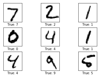
1 2 3 4 5 6 7 8 9 10 11 12 13 14 15 16 17 18 19 20 21 22 23 24 25 26 27 28 29 30 31 32 33 34 35 36 def plot_images (images, cls_true, cls_pred=None ): assert len (images) == len (cls_true) == 9 fig, axes = plt.subplots(3 , 3 ) fig.subplots_adjust(hspace=0.3 , wspace=0.3 ) for i, ax in enumerate (axes.flat): ax.imshow(images[i].reshape(img_shape), cmap='binary' ) if cls_pred is None : xlabel = "True: {0}" .format (cls_true[i]) else : xlabel = "True: {0}, Pred: {1}" .format (cls_true[i], cls_pred[i]) ax.set_xlabel(xlabel) ax.set_xticks([]) ax.set_yticks([]) plt.show() images = data.test.images[0 :9 ] cls_true = data.test.cls[0 :9 ] plot_images(images=images, cls_true=cls_true)
构造训练模型 1 2 3 4 5 6 7 8 9 def new_weights (shape ): ''' 随机产生一个形状为shape的服从截断正态分布 均值为mean,标准差为stddev的tensor 截断的方法根据官方API的定义为 如果单次随机生成的值偏离均值2倍标准差之外 就丢弃并重新随机生成一个新的数。 ''' return tf.Variable(tf.truncated_normal(shape, stddev=0.05 ))
1 2 3 4 5 6 def new_biases (length ): ''' 偏置生成函数,因为激活函数使用的是ReLU 我们给偏置增加一些小的正值(0.05)避免死亡节点(dead neurons) ''' return tf.Variable(tf.constant(0.05 , shape=[length]))
池化层 当输入经过卷积层时,若感受视野比较小,布长stride比较小,得到的feature map (特征图)还是比较大,可以通过池化层来对每一个 feature map 进行降维操作,输出的深度还是不变的,依然为 feature map 的个数。
池化层也有一个 filter 来对feature map矩阵进行扫描,对“池化视野”中的矩阵值进行计算,一般有两种计算方式:
Max pooling:取“池化视野”矩阵中的最大值
Average pooling:取“池化视野”矩阵中的平均值
1 2 3 4 5 6 7 8 9 10 11 12 13 14 15 16 17 18 19 20 21 22 23 24 25 26 27 def new_conv_layer (input , num_input_channels, filter_size, num_filters, use_pooling=True ): shape = [filter_size, filter_size, num_input_channels, num_filters] weights = new_weights(shape) biases = new_biases(num_filters) layer = tf.nn.conv2d(input =input , filter =weights, strides=[1 , 1 , 1 , 1 ], padding='SAME' ) layer += biases if use_pooling: layer = tf.nn.max_pool(value=layer, ksize=[1 , 2 , 2 , 1 ], strides=[1 , 2 , 2 , 1 ], padding='SAME' ) layer = tf.nn.relu(layer) return layer, weights
1 2 3 4 5 6 7 8 9 10 11 12 13 14 def flatten_layer (layer ): layer_shape = layer.get_shape() num_features = layer_shape[1 :4 ].num_elements() layer_flat = tf.reshape(layer, [-1 , num_features]) return layer_flat, num_features
ReLu: $f(x) = max(x, 0)$
1 2 3 4 5 6 7 8 9 10 11 12 def new_fc_layer (input , num_inputs, num_outputs, use_relu=True ): weights = new_weights(shape=[num_inputs, num_outputs]) biases = new_biases(length=num_outputs) layer = tf.matmul(input , weights) + biases if use_relu: layer = tf.nn.relu(layer) return layer
Placeholder variables 1 2 3 4 5 x = tf.placeholder(tf.float32, shape=[None , img_size_flat], name='x' ) x_image = tf.reshape(x, [-1 , img_size, img_size, num_channels]) y_true = tf.placeholder(tf.float32, shape=[None , num_classes], name='y_true' ) y_true_cls = tf.argmax(y_true, axis=1 )
卷积层 1 2 3 4 5 6 7 layer_conv1, weights_conv1 = \ new_conv_layer(input =x_image, num_input_channels=num_channels, filter_size=filter_size1, num_filters=num_filters1, use_pooling=True ) layer_conv1
<tf.Tensor 'Relu:0' shape=(?, 14, 14, 16) dtype=float32>
1 2 3 4 5 6 7 layer_conv2, weights_conv2 = \ new_conv_layer(input =layer_conv1, num_input_channels=num_filters1, filter_size=filter_size2, num_filters=num_filters2, use_pooling=True ) layer_conv2
<tf.Tensor 'Relu_1:0' shape=(?, 7, 7, 36) dtype=float32>
Flatten Layer 我也不知道怎么翻译,作用就是将卷积输出的4维tensor,压缩成2维的tensor,用于输入连接层
1 2 layer_flat, num_features = flatten_layer(layer_conv2) print (layer_flat,num_features)
Tensor("Reshape_1:0", shape=(?, 1764), dtype=float32) 1764
连接层 1 2 3 4 5 layer_fc1 = new_fc_layer(input =layer_flat, num_inputs=num_features, num_outputs=fc_size, use_relu=True ) layer_fc1
<tf.Tensor 'Relu_2:0' shape=(?, 128) dtype=float32>
1 2 3 4 5 layer_fc2 = new_fc_layer(input =layer_fc1, num_inputs=fc_size, num_outputs=num_classes, use_relu=False ) layer_fc2
<tf.Tensor 'add_3:0' shape=(?, 10) dtype=float32>
预测 1 2 y_pred = tf.nn.softmax(layer_fc2) y_pred_cls = tf.argmax(y_pred, axis=1 )
损失优化 1 2 3 4 5 6 cross_entropy = tf.nn.softmax_cross_entropy_with_logits_v2(logits=layer_fc2, labels=y_true) cost = tf.reduce_mean(cross_entropy) optimizer = tf.train.AdamOptimizer(learning_rate=1e-4 ).minimize(cost) correct_prediction = tf.equal(y_pred_cls, y_true_cls) accuracy = tf.reduce_mean(tf.cast(correct_prediction, tf.float32))
跑两步 1 2 3 session = tf.Session() session.run(tf.global_variables_initializer()) train_batch_size = 64
1 2 3 4 5 6 7 8 9 10 11 12 13 14 15 16 17 18 total_iterations = 0 def optimize (num_iterations ): global total_iterations start_time = time.time() for i in range (total_iterations, total_iterations + num_iterations): x_batch, y_true_batch = data.train.next_batch(train_batch_size) feed_dict_train = {x: x_batch, y_true: y_true_batch} session.run(optimizer, feed_dict=feed_dict_train) if i % 100 == 0 : acc = session.run(accuracy, feed_dict=feed_dict_train) msg = "Optimization Iteration: {0:>6}, Training Accuracy: {1:>6.1%}" print (msg.format (i + 1 , acc)) total_iterations += num_iterations end_time = time.time() time_dif = end_time - start_time print ("Time usage: " + str (timedelta(seconds=int (round (time_dif)))))
1 2 3 4 5 6 7 8 def plot_example_errors (cls_pred, correct ): incorrect = (correct == False ) images = data.test.images[incorrect] cls_pred = cls_pred[incorrect] cls_true = data.test.cls[incorrect] plot_images(images=images[0 :9 ], cls_true=cls_true[0 :9 ], cls_pred=cls_pred[0 :9 ])
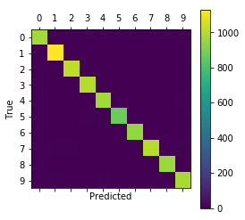
1 2 3 4 5 6 7 8 9 10 11 12 13 def plot_confusion_matrix (cls_pred ): cls_true = data.test.cls cm = confusion_matrix(y_true=cls_true, y_pred=cls_pred) print (cm) plt.matshow(cm) plt.colorbar() tick_marks = np.arange(num_classes) plt.xticks(tick_marks, range (num_classes)) plt.yticks(tick_marks, range (num_classes)) plt.xlabel('Predicted' ) plt.ylabel('True' ) plt.show()
1 2 3 4 5 6 7 8 9 10 11 12 13 14 15 16 17 18 19 20 21 22 23 24 25 26 test_batch_size = 256 def print_test_accuracy (show_example_errors=False , show_confusion_matrix=False ): num_test = len (data.test.images) cls_pred = np.zeros(shape=num_test, dtype=np.int ) i = 0 while i < num_test: j = min (i + test_batch_size, num_test) images = data.test.images[i:j, :] labels = data.test.labels[i:j, :] feed_dict = {x: images, y_true: labels} cls_pred[i:j] = session.run(y_pred_cls, feed_dict=feed_dict) i = j cls_true = data.test.cls correct = (cls_true == cls_pred) correct_sum = correct.sum () acc = float (correct_sum) / num_test msg = "Accuracy on Test-Set: {0:.1%} ({1} / {2})" print (msg.format (acc, correct_sum, num_test)) if show_example_errors: print ("Example errors:" ) plot_example_errors(cls_pred=cls_pred, correct=correct) if show_confusion_matrix: print ("Confusion Matrix:" ) plot_confusion_matrix(cls_pred=cls_pred)
初始数据 <tf.Tensor 'ArgMax_1:0' shape=(?,) dtype=int64>
Accuracy on Test-Set: 10.2% (1016 / 10000)
跑一步 1 2 optimize(num_iterations=1 ) print_test_accuracy()
Optimization Iteration: 1, Training Accuracy: 14.1%
Time usage: 0:00:00
Accuracy on Test-Set: 8.9% (889 / 10000)
跑 100 步 1 2 optimize(num_iterations=99 ) print_test_accuracy()
Time usage: 0:00:04
Accuracy on Test-Set: 63.9% (6388 / 10000)
跑 1000步 1 2 optimize(num_iterations=900 ) print_test_accuracy()
Optimization Iteration: 101, Training Accuracy: 62.5%
Optimization Iteration: 201, Training Accuracy: 78.1%
Optimization Iteration: 301, Training Accuracy: 79.7%
Optimization Iteration: 401, Training Accuracy: 90.6%
Optimization Iteration: 501, Training Accuracy: 92.2%
Optimization Iteration: 601, Training Accuracy: 92.2%
Optimization Iteration: 701, Training Accuracy: 95.3%
Optimization Iteration: 801, Training Accuracy: 85.9%
Optimization Iteration: 901, Training Accuracy: 96.9%
Time usage: 0:00:38
Accuracy on Test-Set: 94.2% (9425 / 10000)
1 print_test_accuracy(show_example_errors=True )
Accuracy on Test-Set: 94.2% (9425 / 10000)
Example errors:
跑10000步 1 2 3 optimize(num_iterations=9000 ) print_test_accuracy(show_example_errors=True , show_confusion_matrix=True )
Optimization Iteration: 1001, Training Accuracy: 87.5%
Optimization Iteration: 7301, Training Accuracy: 100.0%
Optimization Iteration: 7401, Training Accuracy: 100.0%
Optimization Iteration: 9501, Training Accuracy: 98.4%
Optimization Iteration: 9601, Training Accuracy: 100.0%
Optimization Iteration: 9901, Training Accuracy: 96.9%
Time usage: 0:05:44
Accuracy on Test-Set: 98.8% (9876 / 10000)
Example errors:
Confusion Matrix:
[[ 972 0 1 0 0 0 3 1 3 0]
[ 0 1131 1 0 0 0 1 1 1 0]
[ 1 3 1020 1 1 0 0 2 4 0]
[ 0 0 1 1002 0 4 0 1 2 0]
[ 0 0 1 0 975 0 1 0 0 5]
[ 2 1 0 5 0 878 1 0 3 2]
[ 2 2 0 0 3 3 947 0 1 0]
[ 1 5 6 2 0 0 0 1007 1 6]
[ 3 0 1 2 1 0 2 2 961 2]
[ 3 5 0 2 8 4 0 2 2 983]]
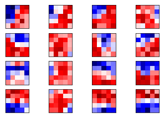
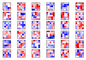
卷积分析 1 2 3 4 5 6 7 8 9 10 11 12 13 14 15 16 17 18 19 20 21 22 def plot_conv_weights (weights, input_channel=0 ): w = session.run(weights) w_min = np.min (w) w_max = np.max (w) num_filters = w.shape[3 ] num_grids = math.ceil(math.sqrt(num_filters)) fig, axes = plt.subplots(num_grids, num_grids) for i, ax in enumerate (axes.flat): if i< num_filters: img = w[:, :, input_channel, i] ax.imshow(img, vmin=w_min, vmax=w_max, interpolation='nearest' , cmap='seismic' ) ax.set_xticks([]) ax.set_yticks([]) plt.show() plot_conv_weights(weights=weights_conv1)
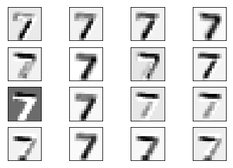
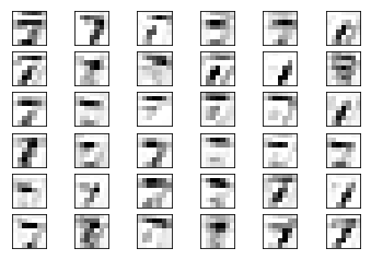
1 2 3 4 5 6 7 8 9 10 11 12 13 14 def plot_conv_layer (layer, image ): feed_dict = {x : [image]} values = session.run(layer, feed_dict=feed_dict) num_filters = values.shape[3 ] num_grids = math.ceil(math.sqrt(num_filters)) fig, axes = plt.subplots(num_grids, num_grids) for i, ax in enumerate (axes.flat): if i<num_filters: img = values[0 , :, :, i] ax.imshow(img, interpolation='nearest' , cmap='binary' ) ax.set_xticks([]) ax.set_yticks([]) plt.show() plot_conv_layer(layer=layer_conv1, image=data.test.images[0 ])
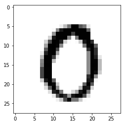
1 2 3 4 5 def plot_image (image ): plt.imshow(image.reshape(img_shape), interpolation='nearest' , cmap='binary' ) plt.show()
1 2 image1 = data.test.images[0 ] plot_image(image1)
1 2 image2 = data.test.images[13 ] plot_image(image2)
第一层卷积 <tf.Variable 'Variable:0' shape=(5, 5, 1, 16) dtype=float32_ref>
1 plot_conv_weights(weights=weights_conv1)
1 2 3 plot_conv_layer(layer=layer_conv1, image=image1)
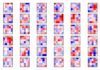
卷积层2 1 plot_conv_weights(weights=weights_conv2, input_channel=0 )
1 plot_conv_weights(weights=weights_conv2, input_channel=1 )
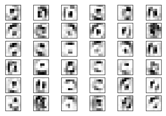
1 plot_conv_layer(layer=layer_conv2, image=image1)
1 plot_conv_layer(layer=layer_conv2, image=image2)