TensorFlow Tutorial

上一篇教程写的实在是有点看不下去，重新写一个吧。

开始

导入相关包

%matplotlib inline
import matplotlib.pyplot as plt
import tensorflow as tf
import numpy as np
from sklearn.metrics import confusion_matrix

获取MNIST数据集

from tensorflow.examples.tutorials.mnist import input_data
data = input_data.read_data_sets("data/MNIST_data/", one_hot=True)

MNIST的信息

print("Size of:")
print("- Training-set:\t\t{}".format(len(data.train.labels)))
print("- Test-set:\t\t{}".format(len(data.test.labels)))
print("- Validation-set:\t{}".format(len(data.validation.labels)))

Size of:
- Training-set:        55000
- Test-set:        10000
- Validation-set:    5000

print(data.test.labels[0:5, :])
data.test.cls = np.array([label.argmax() for label in data.test.labels])
print(data.test.cls)
print(data.test.cls[0:5])

[[0. 0. 0. 0. 0. 0. 0. 1. 0. 0.]
 [0. 0. 1. 0. 0. 0. 0. 0. 0. 0.]
 [0. 1. 0. 0. 0. 0. 0. 0. 0. 0.]
 [1. 0. 0. 0. 0. 0. 0. 0. 0. 0.]
 [0. 0. 0. 0. 1. 0. 0. 0. 0. 0.]]
[7 2 1 ... 4 5 6]
[7 2 1 0 4]

# 图片大小
img_size = 28
# 当图片一维保存时的长度
img_size_flat = img_size * img_size
# 图片的形状 Tuple
img_shape = (img_size, img_size)
# 种类的数量，比如数字识别就是0~9 10个种类，猫狗识别就只有 2个类型
num_classes = 10

# 画图
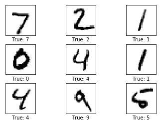
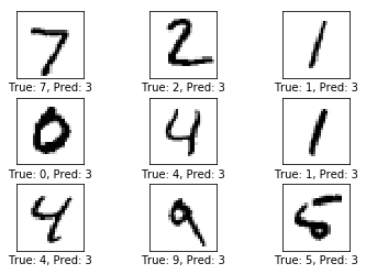
def plot_images(images, cls_true, cls_pred=None):
    assert len(images) == len(cls_true) == 9
    # 造一个3 x 3 的格子
    fig, axes = plt.subplots(3,3)
    fig.subplots_adjust(hspace=0.3, wspace=0.3)
    for i, ax in enumerate(axes.flat):
        # 黑白画图
        ax.imshow(images[i].reshape(img_shape), cmap='binary')
        if cls_pred is None:
            xlabel = "True: {0}".format(cls_true[i])
        else:
            xlabel = "True: {0}, Pred: {1}".format(cls_true[i],cls_pred[i])
        # 设置x周标记
        ax.set_xlabel(xlabel)
        # 清理横纵坐标
        ax.set_xticks([])
        ax.set_yticks([])
    plt.show()

images = data.test.images[0:9]
cls_true = data.test.cls[0:9]
plot_images(images=images, cls_true=cls_true)

初始Tensorflow模型

# 图像
x = tf.placeholder(tf.float32, [None, img_size_flat])
# 真实值，one hot 编码的
y_true = tf.placeholder(tf.float32, [None, num_classes])
# 真实值标签 argmax之后的 y_true
y_true_cls = tf.placeholder(tf.int64, [None])

除了上面定义向模型提供输入数据的 placeholder，还有一些由 Tensorflow 训练获得的值。

这两个其实不一样，placeholder是原始数据，训练的时候不变。Variable 是训练的时候的哪些变量。

# 初始权重， img_size_flat x num_classes 大小的一个举证，初始值为0
weights = tf.Variable(tf.zeros([img_size_flat, num_classes]))
# 偏差，其实就是预测值和真实值的差，所以是一维的一个参数
biases = tf.Variable(tf.zeros([num_classes]))

定义线性模型，logits = x * weights + biases ， x 是 [num_images, img_size_flat]， weights 是 [img_size_flat, num_classes], biases 是 [num_classes]， 所以 logits 是一个 [num_images, num_classes]。

换句话说， 每一个images，都有一个对应的class

logits = tf.matmul(x, weights) + biases
# softmax处理数值，使数值分布在0~1之间。
y_pred = tf.nn.softmax(logits)
y_pred_cls = tf.argmax(y_pred, axis=1)

# 定义 cross_entropy
cross_entropy = tf.nn.softmax_cross_entropy_with_logits_v2 \
                    (logits=logits, labels=y_true)
# 取均值
cost = tf.reduce_mean(cross_entropy)

# 优化器
optimizer = tf.train.GradientDescentOptimizer(learning_rate=0.5)\
                .minimize(cost)
# 预测准确度
correct_prediction = tf.equal(y_pred_cls, y_true_cls)
# 准确度
# tf.cast(x, dtype, name=None) 类型转换函数
# x：输入
# dtype：转换目标类型
# name：名称
accuracy = tf.reduce_mean(tf.cast(correct_prediction, tf.float32))

TensorFlow 跑两步

session = tf.Session()
# 初始全部的变量
session.run(tf.global_variables_initializer())
# 50000个图直接跑太费事儿，所以使用随机梯度下降算法，每次跑100个图
# 小步快跑
batch_size = 100

def optimize(num_iterations):
    for i in range(num_iterations):
        x_batch, y_true_batch = data.train.next_batch(batch_size)
        feed_dict_train = {x : x_batch,
                          y_true: y_true_batch}
        session.run(optimizer, feed_dict=feed_dict_train)

feed_dict_test = {x: data.test.images,
                 y_true: data.test.labels,
                 y_true_cls: data.test.cls}

# 这个准确率跟乱猜也差不多。。。
def print_accuracy():
    acc = session.run(accuracy, feed_dict=feed_dict_test)
    print("测试集准确率: {0:.1%}".format(acc))
print_accuracy()

测试集准确率: 9.8%

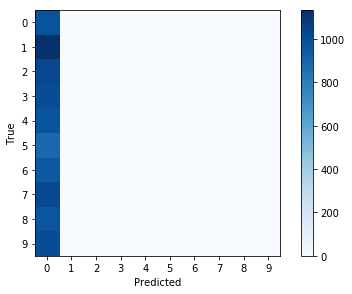
def print_confusion_matrix():
    cls_true = data.test.cls
    cls_pred = session.run(y_pred_cls, feed_dict=feed_dict_test)
    # Get the confusion matrix using sklearn.
    cm = confusion_matrix(y_true=cls_true,
                          y_pred=cls_pred)
    # 输出confusion_matrix矩阵
    print(cm)
    # 画对应的图
    plt.imshow(cm, interpolation='nearest', cmap=plt.cm.Blues)
    
    # 略微调整一下
    plt.tight_layout()
    plt.colorbar()
    tick_marks = np.arange(num_classes)
    plt.xticks(tick_marks, range(num_classes))
    plt.yticks(tick_marks, range(num_classes))
    plt.xlabel('Predicted')
    plt.ylabel('True')
    
    plt.show()    
print_confusion_matrix()

[[ 980    0    0    0    0    0    0    0    0    0]
 [1135    0    0    0    0    0    0    0    0    0]
 [1032    0    0    0    0    0    0    0    0    0]
 [1010    0    0    0    0    0    0    0    0    0]
 [ 982    0    0    0    0    0    0    0    0    0]
 [ 892    0    0    0    0    0    0    0    0    0]
 [ 958    0    0    0    0    0    0    0    0    0]
 [1028    0    0    0    0    0    0    0    0    0]
 [ 974    0    0    0    0    0    0    0    0    0]
 [1009    0    0    0    0    0    0    0    0    0]]

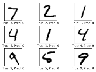
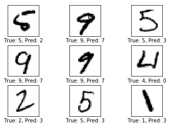
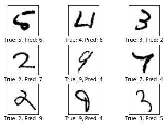
def plot_example_errors():
    correct, cls_pred = session.run([correct_prediction, y_pred_cls],
                                   feed_dict=feed_dict_test)
    incorrect = (correct == False)
    images = data.test.images[incorrect]
    cls_pred = cls_pred[incorrect]
    cls_true = data.test.cls[incorrect]
    plot_images(images[0:9],
               cls_true[0:9],
               cls_pred[0:9])
plot_example_errors()

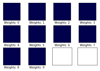
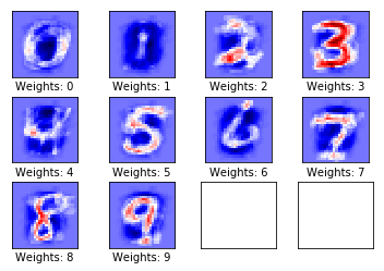
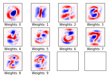
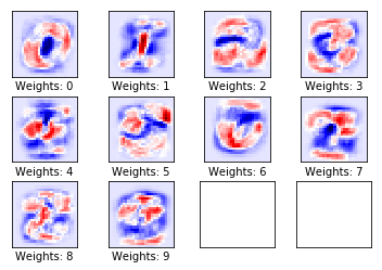
def plot_weights():
    w = session.run(weights)
    w_min = np.min(w)
    w_max = np.max(w)
    # 画格子，调整边距
    fig, axes = plt.subplots(3, 4)
    fig.subplots_adjust(hspace=0.3, wspace=0.3)
    
    for i, ax in enumerate(axes.flat):
        if i<10:
            image = w[:, i].reshape(img_shape)
            ax.set_xlabel("Weights: {}".format(i))
            ax.imshow(image, vmin=w_min, vmax=w_max, cmap='seismic')
        ax.set_xticks([])
        ax.set_yticks([])
    plt.show()
plot_weights()

跑一步

optimize(num_iterations=1)
print_accuracy()
plot_example_errors()
plot_weights()

测试集准确率: 11.7%

跑10步

optimize(num_iterations=9)
print_accuracy()
plot_example_errors()
plot_weights()

测试集准确率: 81.1%

跑1000步

optimize(num_iterations=990)
print_accuracy()
plot_example_errors()
plot_weights()

测试集准确率: 91.9%

print_confusion_matrix()

[[ 958    0    3    2    0    6    8    1    2    0]
 [   0 1094    2    2    1    1    4    2   29    0]
 [   5    7  914   18   13    4   11   10   44    6]
 [   3    0   15  917    0   28    3   11   27    6]
 [   1    1    6    1  922    0    9    2   12   28]
 [   9    1    4   40   10  761   17    6   37    7]
 [  11    3    6    1   12   12  906    1    6    0]
 [   3    7   21    8    7    1    0  944    6   31]
 [   4    4    5   15    9   22    9    8  894    4]
 [   9    4    3    9   51    6    0   27   16  884]]

session.close()

结论

线性模型的准确率约为： 91.9% ，堪忧啊，还要再搏一搏。