天池 ·【新人赛】工业蒸汽量预测建模算法【一】
题目链接 【新人赛】工业蒸汽量预测建模算法,使用线性回归、DNN、CNN进行推荐。
数据分析
读取原始数据并分类
1 | train_data_path = "data/zhengqi_train.txt" |
训练集、评估集、测试集
查看相关性
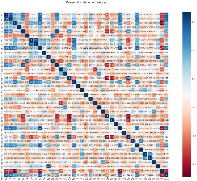
关于热力图的画法 请参考1
2fig, ax = plt.subplots(figsize=(10,10)) # Sample figsize in inches
sns.heatmap(train_df.iloc[:,2:].corr(), annot=True, fmt = ".2f", cmap = "coolwarm", ax=ax)
感觉
1 | source_data.describe() |
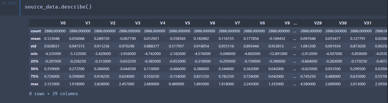
数据偏简单,而且没有空的部分,可做的特征处理不多。
linear 模型
1 | # Parameters |
训练完模型,看看效果1
print(metrics.mean_squared_error(sess.run(pred, feed_dict={x: evaluate}),evaluate_target))
0.9953607
好吧,再回忆一下 热力图,可能的确不怎么适合用线性模型。
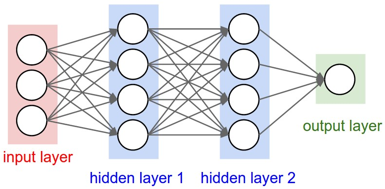
DNN 模型
1
2
3
4
5
6
7
8
9
10
11
12
13
14
15
16
17
18
19
20
21
22
23
24
25
26
27
28
29
30
31
32
33
34
35
36
37
38
39
40
41
42
43
44
45
46
47
48
49
50
51
52
53
54
55
56
57ops.reset_default_graph()
# Parameters
learning_rate = 0.1
num_steps = 10000
batch_size = 100
display_step = 1000
# Network Parameters
n_hidden_1 = 64 # 1st layer number of neurons
n_hidden_2 = 256 # 2nd layer number of neurons
num_input = train.shape[1] # data input
num_classes = 1
# tf Graph Input
x = tf.placeholder(tf.float32, [None, train.shape[1]], name="x")
y = tf.placeholder(tf.float32, [None], "y")
with tf.variable_scope("dnn"):
w1 = tf.get_variable(name="w1", shape=[num_input, n_hidden_1],
initializer=tf.contrib.layers.xavier_initializer())
b1 = tf.get_variable(name="b1", shape=[n_hidden_1],
initializer=tf.contrib.layers.xavier_initializer())
layer_1 = tf.nn.softmax(tf.add(tf.matmul(x, w1), b1))
w2 = tf.get_variable(name="w2", shape=[n_hidden_1, n_hidden_2],
initializer=tf.contrib.layers.xavier_initializer())
b2 = tf.get_variable(name="b2", shape=[n_hidden_2],
initializer=tf.contrib.layers.xavier_initializer())
layer_2 = tf.nn.softmax(tf.add(tf.matmul(layer_1, w2), b2))
w3 = tf.get_variable(name="w3", shape=[n_hidden_2, num_classes],
initializer=tf.contrib.layers.xavier_initializer())
b3 = tf.get_variable(name="b3", shape=[num_classes],
initializer=tf.contrib.layers.xavier_initializer())
pred = tf.add(tf.matmul(layer_2, w3), b3)
# Mean squared error
cost = tf.reduce_sum(tf.pow(pred-y, 2))/len(train)
# Gradient descent
optimizer = tf.train.AdagradOptimizer(learning_rate).minimize(cost)
sess = tf.Session()
# Initialize the variables (i.e. assign their default value)
sess.run(tf.global_variables_initializer())
for step in range(num_steps):
if train.shape[0] == batch_size:
batch_start_idx = 0
else:
batch_start_idx = (i * batch_size) % (train.shape[0] - batch_size)
batch_end_idx = batch_start_idx + batch_size
xs = train[batch_start_idx:batch_end_idx]
ys = train_target[batch_start_idx:batch_end_idx]
sess.run(optimizer, feed_dict={ x: xs, y: ys })
if step % display_step == 0 or step == 1:
print("steps:{},cost:{}".format(step, sess.run(cost,feed_dict = {x: train, y: train_target})))
输出是:1
2
3
4
5
6
7
8
9
10
11steps:0,cost:2083.156005859375
steps:1,cost:2014.62158203125
steps:1000,cost:1947.38623046875
steps:2000,cost:1947.38623046875
steps:3000,cost:1947.38623046875
steps:4000,cost:1947.38623046875
steps:5000,cost:1947.38623046875
steps:6000,cost:1947.38623046875
steps:7000,cost:1947.38623046875
steps:8000,cost:1947.38623046875
steps:9000,cost:1947.38623046875
预测一下吧:1
print(metrics.mean_squared_error(sess.run(pred, feed_dict={x: evaluate}),evaluate_target))
1.0276294
还真是… 这种简单问题,用DNN不一定合适。
CNN
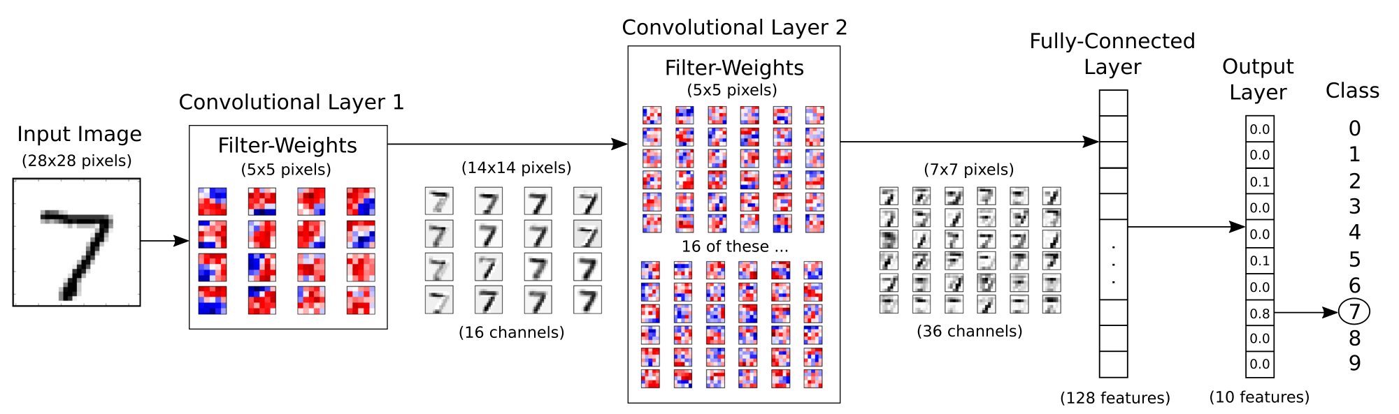
图仅供释义1
2
3
4
5
6
7
8
9
10
11
12
13
14
15
16
17
18
19
20
21
22
23
24
25
26
27
28
29
30
31
32
33
34
35
36
37
38
39
40
41
42
43
44
45
46
47
48
49
50
51
52
53
54
55
56
57
58
59
60
61
62
63
64
65
66
67
68
69
70
71
72
73
74
75
76
77
78
79
80
81
82
83
84
85
86
87
88
89
90
91
92
93
94
95
96
97
98
99
100
101
102
103ops.reset_default_graph()
# Parameters
learning_rate = 0.001
num_steps = 10000
batch_size = 100
display_step = 1000
# 卷积核大小
filter_size1 = 5
# 16个卷积核
num_filters1 = 16
filter_size2 = 5
num_filters2 = 36
# 全连接层 神经元数目。
fc_size = 128
# tf Graph Input
x = tf.placeholder(tf.float32, [None, train.shape[1]], name="x")
# 标准输入格式[个数,长,宽,高],因为CNN主要是做图像处理的
# 这里的高 指的就是维度,比如彩色就是3维,黑白就是1维
# 在推荐系统中,没有长和高这么一说,所以增加两个维度
input_layer = tf.expand_dims(x, 1)
input_layer = tf.expand_dims(input_layer, 3)
y = tf.placeholder(tf.float32, [None], "y")
keep_prob = tf.placeholder(tf.float32)
with tf.variable_scope("cnn"):
# 卷积层1
# shape[长,宽,入通道数,filter个数/出通道数]
w1 = tf.get_variable("filterW1", shape=[1, filter_size1, 1, num_filters1],
initializer=tf.contrib.layers.xavier_initializer())
b1 = tf.get_variable("filterB1", shape=[num_filters1])
# stride 参考: https://iii.run/archives/138.html#directory087197468524675785
# padding 参考: https://iii.run/archives/138.html#directory087197468524675786
conv1 = tf.nn.conv2d(input_layer,w1,strides=[1, 1, 3, 1],
padding="SAME",name="layer1")
conv1 = tf.nn.bias_add(conv1, b1)
conv1 = tf.nn.relu(conv1)
# 池化层
conv1 = tf.nn.max_pool(value=conv1, ksize=[1, 1, 2, 1],
strides=[1, 1, 2, 1],padding='SAME')
# 卷积层2
w2 = tf.get_variable("filterW2", shape=[1, filter_size1, num_filters1, num_filters2],
initializer=tf.contrib.layers.xavier_initializer())
b2 = tf.get_variable("filterB2", shape=[num_filters2])
conv2 = tf.nn.conv2d(conv1, w2, strides=[1, 1, 3, 1],
padding="SAME", name="layer2")
conv2 = tf.nn.bias_add(conv2, b2)
# 用 relu也行,据说sigmoid效果比relu好,但是sigmoid非常慢
conv2 = tf.nn.sigmoid(conv2)
# 减少过拟合程度,丢弃某些神经元的输出结果
conv2 = tf.nn.dropout(conv2, keep_prob)
conv2_shape = conv2.get_shape().as_list()
# 全连接层
with tf.variable_scope("full_connect"):
w_fc1 = tf.get_variable("w_fc1", shape=[conv2_shape[2] * conv2_shape[3], fc_size],
initializer=tf.contrib.layers.xavier_initializer())
b_fc1 = tf.get_variable("b_fc1", shape=[fc_size],
initializer=tf.contrib.layers.xavier_initializer())
conv2_flat = tf.reshape(conv2, [-1, conv2_shape[2] * conv2_shape[3]])
fc1_out = tf.nn.relu(tf.matmul(conv2_flat, w_fc1) + b_fc1)
# 输出层
with tf.variable_scope("out"):
w_fc2 = tf.get_variable("w_fc2", shape=[fc_size,1],
initializer=tf.contrib.layers.xavier_initializer())
b_fc2 = tf.get_variable("b_fc2", shape=[1],
initializer=tf.contrib.layers.xavier_initializer())
# 与 fc2_out = tf.nn.matmul(fc1_out,w_fc2)+b_fc2 同义
fc2_out = tf.nn.xw_plus_b(fc1_out,w_fc2,b_fc2)
pred = fc2_out
# 定义优化目标
# Mean squared error
cost = tf.reduce_sum(tf.pow(pred-y, 2))/len(train)
# Gradient descent
optimizer = tf.train.AdagradOptimizer(learning_rate).minimize(cost)
sess = tf.Session()
# Initialize the variables (i.e. assign their default value)
sess.run(tf.global_variables_initializer())
for step in range(num_steps):
if train.shape[0] == batch_size:
batch_start_idx = 0
else:
batch_start_idx = (i * batch_size) % (train.shape[0] - batch_size)
batch_end_idx = batch_start_idx + batch_size
xs = train[batch_start_idx:batch_end_idx]
ys = train_target[batch_start_idx:batch_end_idx]
sess.run(optimizer, feed_dict={ x: xs, y: ys,keep_prob:0.5})
if step % display_step == 0 or step == 1:
print("steps:{},cost:{}".format(step, sess.run(cost,feed_dict = {x: train, y: train_target,keep_prob:0.5})))
输出1
2
3
4
5
6
7
8
9
10
11steps:0,cost:3606.652587890625
steps:1,cost:3139.012939453125
steps:1000,cost:2025.926513671875
steps:2000,cost:1998.60986328125
steps:3000,cost:1992.10205078125
steps:4000,cost:1984.5877685546875
steps:5000,cost:1979.1214599609375
steps:6000,cost:1974.5855712890625
steps:7000,cost:1976.9493408203125
steps:8000,cost:1972.7890625
steps:9000,cost:1973.3104248046875
看一下测试集的效果1
print(metrics.mean_squared_error(sess.run(pred, feed_dict={x: evaluate,keep_prob:0.5}),evaluate_target))
1.0461832
小结
对于简单的推荐问题,线性回归>DNN>CNN,越复杂的方案效果越不好。
用到的python包
1 | import tensorflow as tf |
天池 ·【新人赛】工业蒸汽量预测建模算法【一】