Coursera ML(4)-Logistic Regression

本节笔记对应第三周Coursera课程 binary classification problem

---

Classification is not actually a linear function.

Classification and Representation

Hypothesis Representation

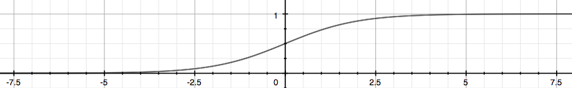
• Sigmoid Function(or we called Logistic Function) $$\begin{align*}& h_\theta (x) = g ( \theta^T x ) \newline \newline& z = \theta^T x \newline& g(z) = \dfrac{1}{1 + e^{-z} }\end{align*}$$ Sigmoid Function 可以使输出值范围在$(0,1)$之间。$g(z)$对应的图为：
  

• $h_\theta(x)$ will give us the probability that our output is 1.
• Some basic knowledge of discrete $$\begin{align*}& h_\theta(x) = P(y=1 | x ; \theta) = 1 - P(y=0 | x ; \theta) \newline& P(y = 0 | x;\theta) + P(y = 1 | x ; \theta) = 1\end{align*}$$

Decision Boundary

• translate the output of the hypothesis function as follows: $$\begin{align*}& h_\theta(x) \geq 0.5 \rightarrow y = 1 \newline& h_\theta(x) < 0.5 \rightarrow y = 0 \newline\end{align*}$$
• From these statements we can now say: $$\begin{align*}& \theta^T x \geq 0 \Rightarrow y = 1 \newline& \theta^T x < 0 \Rightarrow y = 0 \newline\end{align*}$$

Logistic Regression Model

Cost function for one variable hypothesis

• To let the cost function be convex for gradient descent, it should be like this: $$J(\theta) = \dfrac{1}{m} \sum_{i=1}^m \mathrm{Cost}(h_\theta(x^{(i)}),y^{(i)})$$

$$Cost(h_\theta (x), y) =\begin{cases}-log(h_\theta (x)), (y = 1) \\-log(1 - h_\theta (x)), (y = 0) \\\end{cases}$$

• example $$\begin{align*}& \mathrm{Cost}(h_\theta(x),y) = 0 \text{ if } h_\theta(x) = y \newline & \mathrm{Cost}(h_\theta(x),y) \rightarrow \infty \text{ if } y = 0 \; \mathrm{and} \; h_\theta(x) \rightarrow 1 \newline & \mathrm{Cost}(h_\theta(x),y) \rightarrow \infty \text{ if } y = 1 \; \mathrm{and} \; h_\theta(x) \rightarrow 0 \newline \end{align*}$$

Simplified Cost Function and Gradient Descent

• compress our cost function’s two conditional cases into one case:

  $$\mathrm{Cost}(h_\theta(x),y) = - y \; \log(h_\theta(x)) - (1 - y) \log(1 - h_\theta(x))$$

• entire cost function

  $$J(\theta) = - \frac{1}{m} \displaystyle \sum_{i=1}^m [y^{(i)}\log (h_\theta (x^{(i)})) + (1 - y^{(i)})\log (1 - h_\theta(x^{(i)}))]$$

Gradient Descent

• the general form of gradient descent ，求偏导的得到$J(\theta)$的极值

  $$\begin{align*}& Repeat \; \lbrace \newline & \; \theta_j := \theta_j - \alpha \dfrac{\partial}{\partial \theta_j}J(\theta) \newline & \rbrace\end{align*}$$

• using calculus

  $$\frac{\partial}{\partial \theta_j} J(\theta) = \frac{1}{m}\sum\limits_{i=1}^{m}[(h_\theta (x^{(i)}) - y^{(i)})x_j^{(i)}]$$

• get

  $$\begin{align*} & Repeat \; \lbrace \newline & \; \theta_j := \theta_j - \frac{\alpha}{m} \sum_{i=1}^m (h_\theta(x^{(i)}) - y^{(i)}) x_j^{(i)} \newline & \rbrace \end{align*}$$

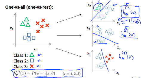
Multiclass Classification: One-vs-all

• For more than 2 features of y, do logisitc regression for each feature separately
• Train a logistic regression classifier $h_\theta(x)$ for each class to predict the probability that  y = i .
• To make a prediction on a new x, pick the class that maximizes $ h_\theta (x) $
  

Solving the Problem of Overfitting

The Problem of Overfitting

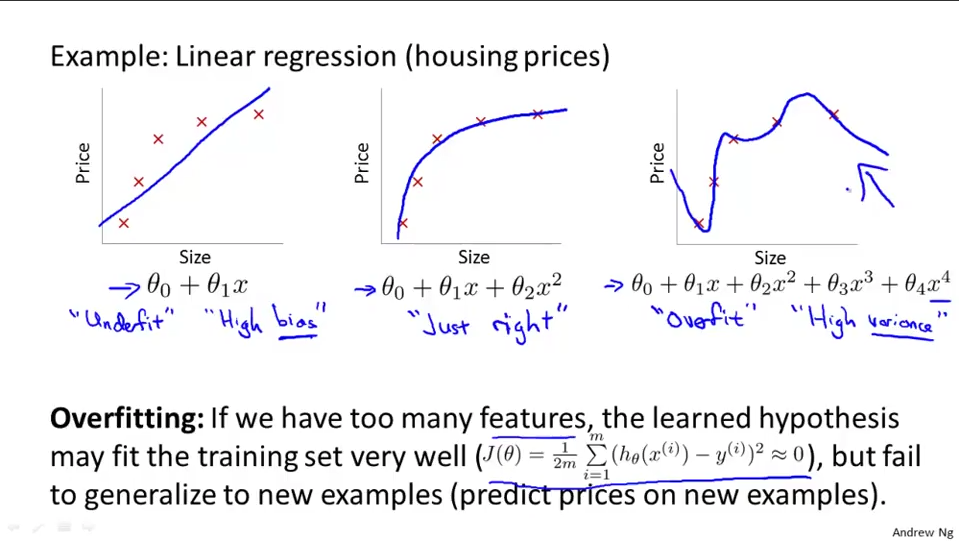
address the issue of overfitting

• Reduce the number of features:
  • Manually select which features to keep.
  • Use a model selection algorithm (studied later in the course).
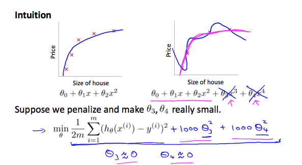
• Regularization:
  • Keep all the features, but reduce the magnitude of parameters $θ_j$.
  • Regularization works well when we have a lot of slightly useful features.

Cost Function

• in a single summation $$min_\theta\ \dfrac{1}{2m}\ \sum_{i=1}^m (h_\theta(x^{(i)}) - y^{(i)})^2 + \lambda\ \sum_{j=1}^n \theta_j^2$$

The λ, or lambda, is the regularization parameter. It determines how much the costs of our theta parameters are inflated.

Regularized Linear Regression

• Gradient Descent

  $$\begin{align*} & \text{Repeat}\ \lbrace \newline & \ \ \ \ \theta_0 := \theta_0 - \alpha\ \frac{1}{m}\ \sum_{i=1}^m (h_\theta(x^{(i)}) - y^{(i)})x_0^{(i)} \newline & \ \ \ \ \theta_j := \theta_j - \alpha\ \left[ \left( \frac{1}{m}\ \sum_{i=1}^m (h_\theta(x^{(i)}) - y^{(i)})x_j^{(i)} \right) + \frac{\lambda}{m}\theta_j \right] &\ \ \ \ \ \ \ \ \ \ j \in \lbrace 1,2...n\rbrace\newline & \rbrace \end{align*}$$

• Normal Equation

  $$\begin{align*}& \theta = \left( X^TX + \lambda \cdot L \right)^{-1} X^Ty \newline& \text{where}\ \ L = \begin{bmatrix} 0 & & & & \newline & 1 & & & \newline & & 1 & & \newline & & & \ddots & \newline & & & & 1 \newline\end{bmatrix}\end{align*}$$
  • L is a matrix with 0 at the top left and 1’s down the diagonal, with 0’s everywhere else. It should have dimension (n+1)×(n+1)
  • Recall that if m ≤ n, then $X^TX$ is non-invertible. However, when we add the term λ⋅L, then $X^TX + λ⋅L $becomes invertible.

Summary

我在这里整理一下上述两个方法，补全课程上的相关推导。

Logistic Regression Model

$h_\theta(x)$是假设函数

$$h_\theta (x) = g ( \theta^T x ) = \dfrac{1}{1 + e^{- \theta^T x} }$$

注意假设函数和真实数据之间的区别

Cost Function

$$J(\theta) = - \frac{1}{m} \sum_{i=1}^m \large[ y^{(i)}\ \log (h_\theta (x^{(i)})) + (1 - y^{(i)})\ \log (1 - h_\theta(x^{(i)}))\large]$$

回头看看上边的那个$h_\theta (x)$ ，cost function定义了训练集给出的结果 和 当前计算结果之间的差距。当然，该差距越小越好，那么需要求导一下。

Gradient Descent

• 原始公式 $$\theta_j := \theta_j - \alpha \dfrac{\partial}{\partial \theta_j}J(\theta)$$
• 求导计算 $$\frac{\partial}{\partial \theta_j} J(\theta) = \frac{1}{m}\sum\limits_{i=1}^{m}[(h_\theta (x^{(i)}) - y^{(i)})x_j^{(i)}]$$
• 计算结果 $$\theta_j := \theta_j - \frac{\alpha}{m} \sum_{i=1}^m (h_\theta(x^{(i)}) - y^{(i)}) x_j^{(i)}$$

这里推导一下$\frac{\partial}{\partial \theta_j} J(\theta)$：

• 计算$h_\theta’(x)$导数

  $$\begin{align*} &h_\theta'(x) = ( \frac1{1+e^{- \theta x} })'\newline &\ \ \ \ \ \ \ \ = \frac{e^{- \theta x}x}{1+e^{- \theta x} }\newline &\ \ \ \ \ \ \ \ = \frac{1+e^{- \theta x}-1}{(1+e^{- \theta x})^2}x\newline &\ \ \ \ \ \ \ \ = \large[\frac{1}{1+e^{- \theta x} }-\frac{1}{(1+e^{- \theta x})^2}\large]x\newline &\ \ \ \ \ \ \ \ = h_\theta(x)(1-h_\theta(x))x \end{align*}$$

• 推导$\frac{\partial}{\partial \theta_j} J(\theta)$

$$\begin{align*} &\frac{\partial}{\partial \theta_j} J(\theta) = \frac{\partial}{\partial \theta_j} \frac{1}{m} \sum_{i=1}^m \large[ -y^{(i)}\ \log (h_\theta (x^{(i)})) - (1 - y^{(i)})\ \log (1 - h_\theta(x^{(i)}))\large] \newline &\ \ \ \ \ \ \ \ \ \ \ \ \ \ = \frac{1}{m} \sum_{i=1}^m \large[ -y^{(i)}\ \frac1{h_\theta(x^{(i)})}h_\theta'(x^{(i)}) - (1 - y^{(i)}) \frac{-1}{1-h_\theta(x^{(i)})}h_\theta'(x^{(i)})\large] \newline &\ \ \ \ \ \ \ \ \ \ \ \ \ \ = \frac{1}{m} \sum_{i=1}^m \large[ -y^{(i)}\ \frac1{h_\theta(x^{(i)})}h_\theta(x^{(i)})(1-h_\theta(x^{(i)}))x^{(i)} \newline &\ \ \ \ \ \ \ \ \ \ \ \ \ \ \ \ \ \ \ \ \ \ \ \ \ \ \ \ \ \ \ \ \ \ \ \ \ \ \ \ \ \ \ \ \ \ \ \ \ \ \ - (1 - y^{(i)}) \frac{-1}{1-h_\theta(x^{(i)})}h_\theta(x^{(i)})(1-h_\theta(x^{(i)}))x^{(i)}\large] \newline &\ \ \ \ \ \ \ \ \ \ \ \ \ \ = \frac{1}{m} \sum_{i=1}^m \large[ -y^{(i)}(1-h_\theta(x^{(i)}) x^{(i)})+(1- y)h_\theta(x^{(i)}) x^{(i)})\large] \newline &\ \ \ \ \ \ \ \ \ \ \ \ \ \ = \frac{1}{m} \sum_{i=1}^m \large[ -x^{(i)}y^{(i)}+x^{(i)}y^{(i)}h_\theta(x^{(i)}) \newline &\ \ \ \ \ \ \ \ \ \ \ \ \ \ \ \ \ \ \ \ \ \ \ \ \ \ \ \ \ \ \ \ \ \ \ \ \ \ \ \ \ \ \ \ \ \ \ \ \ \ \ \ \ \ \ \ \ \ \ \ \ \ \ \ \ \ \ \ \ \ \ \ \ \ \ \ \ \ \ \ \ \ \ \ +x^{(i)}h_\theta(x^{(i)}) - x^{(i)}y^{(i)}h_\theta(x^{(i)}) \large] \newline &\ \ \ \ \ \ \ \ \ \ \ \ \ \ = \frac{1}{m}\sum\limits_{i=1}^{m}[(h_\theta (x^{(i)}) - y^{(i)})x_j^{(i)}] \end{align*}$$

即：

$$\begin{align*} &\frac{\partial}{\partial \theta_j} J(\theta) = \frac{1}{m}\sum\limits_{i=1}^{m}[(h_\theta (x^{(i)}) - y^{(i)})x_j^{(i)}] \end{align*}$$

Solving the Problem of Overfitting

其他地方都一样，稍作修改

Cost Function

$$J(\theta) = - \frac{1}{m} \sum_{i=1}^m \large[ y^{(i)}\ \log (h_\theta (x^{(i)})) + (1 - y^{(i)})\ \log (1 - h_\theta(x^{(i)}))\large] + \frac{\lambda}{2m}\sum_{j=1}^n \theta_j^2$$

Gradient Descent

$$\begin{align*} & \text{Repeat}\ \lbrace \newline & \ \ \ \ \theta_0 := \theta_0 - \alpha\ \frac{1}{m}\ \sum_{i=1}^m (h_\theta(x^{(i)}) - y^{(i)})x_0^{(i)} \newline & \ \ \ \ \theta_j := \theta_j - \alpha\ \left[ \left( \frac{1}{m}\ \sum_{i=1}^m (h_\theta(x^{(i)}) - y^{(i)})x_j^{(i)} \right) + \frac{\lambda}{m}\theta_j \right] &\ \ \ \ \ \ \ \ \ \ j \in \lbrace 1,2...n\rbrace\newline & \rbrace \end{align*}$$

---

以上